Probability Distributions

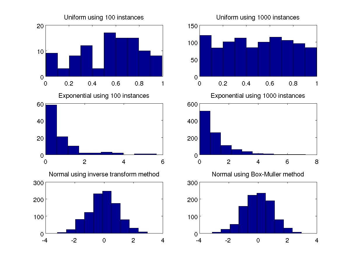
I am playing around with various discrete and continuous distributions for a statistics course assignment. So, I thought of spending few extra minutes and make a matlab script that would plot all of these. Below is the simple matlab script that plots Uniform, Exponential, Normal distributions. The Normal distribution can be generated using inverse transform, box-muller method and the most famous theorem in statistics: The Central Limit theorem.

I want to extend the script to take various parameters and plot more distributions like weibull, poisson etc. but I dont have time right now!

Code:

%% Uniform distribution using 100 instances

u1 = rand(1,100);

%% Uniform distribution using 1000 instances

u2 = rand(1,1000);

%% Exponential distribution using 100 instances

e1 = -log(u1);

%% Exponential distribution using 1000 instances

e2 = -log(u2);

%% Normal distribution using inverse transform method

n1 = norminv(u2,0,1);

%% Normal distribution using box-muller method

n2 = sqrt(-2*log(rand(1,1000))).*cos(2*pi*rand(1,1000));

%% PLOT1 ( Uniform, Exponential, Normal distributions )

figure(1),subplot(3,2,1),hist(u1,10),title('Uniform using 100 instances');

figure(1),subplot(3,2,2),hist(u2,10),title('Uniform using 1000 instances');

figure(1),subplot(3,2,3),hist(e1,10),title('Exponential using 100 instances');

figure(1),subplot(3,2,4),hist(e2,10),title('Exponential using 1000 instances');

figure(1),subplot(3,2,5),hist(n1,10),title('Normal using inverse transform method');

figure(1),subplot(3,2,6),hist(n2,10),title('Normal using Box-Muller method');

%% Triangular distribution

t1 = rand(1,1000);

t2 = rand(1,1000);

t3 = t1 + t2;

%% Central Limit Theorem

n = 12;

for i = 1:n

    t(i,:) = rand(1,1000);

end

n3 = sum(t);

%% PLOT2 ( Trinagular and Normal distributions )

figure(2),subplot(1,2,1),hist(t3),title('Traingular distribution');

figure(2),subplot(1,2,2),hist(n3),title('Normal using central limit theorem');

%% Save to eps files

figure(1),print('-deps','1.eps');

figure(2),print('-deps','2.eps');